
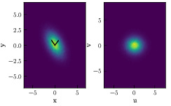
For any linearly correlated distribution there exist a vector which best represents the correlation of its data. We can define such a vector as one which, when data is orthogonally projected onto it, maximizes the variance. It can also be said that it is the vector which minimizes the mean-squared difference between the data and their projected values on to such a vector. This vector is called the first principle component. There is a principle component for every dimension of the sample data, all of which are orthogonal to each other and all of which decrease in magnitude from one to the next.
The principle components can be found by calculating the eigenvectors of the distribution's covariance matrix. Computing a linear transformation in which the data set is multiplied by these eigenvectors will set the principle component vectors as the new basis vectors. This new, transformed, data set will be the most accurate approximation to an uncorrelated distribution.
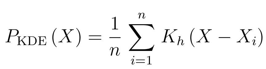
Kernel Density Estimation (KDE) is a more flexible tool which provides a means of extrapolating density from limited sample observation. The kernel, for which the name arrives, is a continuous, non-negative, function where the value of the sample X is a constant in the function. For example,
The functions have a smoothing parameter, h, which is often referred to as the bandwidth. The bandwidth parameter is tuned so that the minimum value can be found to accurately represent the distribution. When tuning the bandwidth there is a trade off between bias and variance. These functions can assume a wide range of values and the dimensionality of them can vary with the needs of the estimation task. A common kernel is the Gaussian kernel,
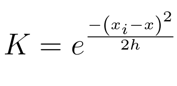
where the sample, x_{i}, represents the well-defined mean of the function and the bandwidth, h, is the standard deviation.
It is common to parameterize the bandwidth by the standard deviation of the data set. This gives sharper functions when the data has lower deviations and broader functions when deviations are larger.
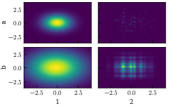
In the above figure a Gaussian distribution is shown as well as a collection of samples drawn from it. Using that sample data, a KDE was used to generate two distributions. In one the bandwidth parameter was set too low, this created a model where the standard deviation is much larger than that of the actual distribution. In the second example, the bandwidth was not set low enough. The bias ended up being much too strong in this case and the distribution barely even resemble a Gaussian. In theory, the KDE should be able to build an extremely good model given that the kernel is the same function as that which was trying to be represented.